I want to move my career in the direction of computer graphics, so lately I’ve been working on a real-time renderer using Vulkan. I won’t make the code public until I consider it portfolio-worthy, but I will publish updates on my progress. Here are the first 14 entries of the offline log I kept.

Entry 0: Hello, world!

2026-10-04

I think it’d be interesting to keep a record of my thoughts, challenges, and what I’ve learned.

I did the Vulkan tutorial 7.5 years ago (https://github.com/LightAndLight/vulkan-hello-triangle) and I remember having to write an exhausting amount of code to get something on the screen. This time around I can still see that it’ll be a solid chunk of code, but I’m less intimidated by it. I think my previous rounds of WebGPU practise (https://blog.ielliott.io/2022-project-review#wgpu-mandelbrot, https://blog.ielliott.io/2023-project-review#3d-graphics-fundamentals) left behind a rough mental model of what’s going on, which has made the Vulkan API feel more approachable. Because of that (and I suppose this is evidence of the confidence I’ve gained) I’m not really following a Vulkan tutorial to get this project off the ground. Let’s see how far I can get with the Vulkan API docs and my prior GPU experience.

What I built

• Started a diagram of the Vulkan API

  I did this previously for WebGPU. I find it really helpful for clarifying the relationships between different parts of the API so that I know what to build next.

• Project setup, build system

• Display a window and enumerate physical devices

What I learned

• Basic CMake configuration

  This is the first time I’ve used CMake in a project. It’s interesting, kind of feels like a relic of another era. I wrote my first CMakeLists.txt and figured out how to provide the dependencies via Nix.

• The precompiled header pattern

  My small windowing program took ~8s to compile every time I changed it. The Vulkan headers were the culprit. Precompiled headers came up as answer and it seemed pretty reasonable so I created one for my project. CMake made it easy to integrate, so I didn’t have to faff around with compiler flags.

• Code samples are helpful

  I’m using Vulkan-Hpp for its RAII wrapper. It doesn’t really have browsable documentation, so it’s hard to search for functions I need. I discovered that the code samples are an okay substitute. For example, I was curious how the apiVersion physical device property was handled, because it’s just a uint32_t. When I searched the samples, I found that Vulkan-Hpp provides macros for extracting the version components. I don’t read code samples very often (I tend to want to figure things out for myself), but after this experience I’m thinking I should do it more often to increase the chance that I’m exposed to good things I didn’t know about before.

Next steps

• Create a swapchain (and all of its dependencies) and start presenting images to the GLFW surface.
• Enable Vulkan Validation Layers in debug builds (remember to trigger some validation failures).

References

• https://docs.vulkan.org/refpages/latest/refpages/

Entry 1: Validation layers and swapchain

2026-10-05

I ran into more trouble than last time, but I’m still feeling pretty comfortable. Very low WTFs/m. Curious about how I’ll go with the graphics pipeline.

The search experience on Vulkan Reference Pages is pretty bad, and I didn’t like that I needed a web browser to read the reference, so I used Claude Opus 5.5 to add a manpage Nix derivation to Vulkan-Docs. This let me read the Vulkan reference using man in my Nix dev shell. This was satisfying for a while, but now I have a couple of gripes:

• apropos doesn’t work in this setting, so I have to get the man argument exactly right.
• man underlines references to other pages, but has no way to navigate to them directly.

So I’ll probably switch back to a HTML reference at some point (unless there’s a good way to do hypertext in the terminal). But it won’t be the official Vulkan reference site.

What I built

• Added Vulkan Validation Layers and fixed all validation errors
• Created a device with a single graphics queue, and a swapchain for the GLFW surface
• Present a swapchain image at ~60Hz

What I learned

• How to provide layers to the Vulkan loader

  I was stumped on this for a while, but after some clicking around I found VK_LAYER_PATH in https://github.com/KhronosGroup/Vulkan-Loader/blob/b82e310e99c20bfac8dd3123c9e939f81ce54b89/docs/LoaderLayerInterface.md#layer-discovery.

  I originally set

  VK_LAYER_PATH = "${pkgs.vulkan-validation-layers}/share";

  in the dev shell, thinking that this rule:

  The directory lists are concatenated together using the standard platform path separator (:). The loader then selects each path, and applies a suffix onto it for the specific type of layer being searched for and looks in that specific folder for manifest files:

  • Implicit Layers: Suffix = /vulkan/implicit_layer.d
  • Explicit Layers: Suffix = /vulkan/explicit_layer.d

  would be applied (${pkgs.vulkan-validation-layers}/share contains vulkan/explicit_layer.d). But I still got a missing layer error.

  I ran the program under strace, which confirmed that the contents of VK_LAYER_PATH were being examined. After re-reading the description of VK_LAYER_PATH:

  If VKLAYERPATH is defined, then the loader will look at the paths defined by that variable for explicit layer manifest files instead of using the information provided by the standard explicit layer paths mentioned above.

  it occurred to me that maybe “look [..] for explicit layer manifest files” meant I should use the full path to manifest file:

  VK_LAYER_PATH = "${pkgs.vulkan-validation-layers}/share/vulkan/explicit_layer.d";

  That worked.

• Vulkan Validation Layers isn’t a panacea

  I got a segfault when creating the swapchain but there were no validation errors. A web search brought me to https://www.reddit.com/r/vulkan/comments/fg2xpy/the_validation_layer_fails_to_report_that_the_vk/, which had the correct diagnosis of my issue. Adding the device-level VK_KHR_swapchain extension fixed it.

  How could I have diagnosed this issue on my own? I tried stepping through with GDB, but there were so… many… calls…

• Vulkan is extremely parallel

  Working with the swapchain required a semaphore, so I read https://www.khronos.org/blog/understanding-vulkan-synchronization to get a handle on the synchronisation primitives.

  My takeaway is that Vulkan is designed to maximise parallelism, so any ordering requirements must be set by the programmer.

Next steps

• Set up a graphics pipeline and draw something to the swapchain image

Entry 2: Graphics pipeline setup

2026-10-06

Today was a bit harder. The Vulkan graphics pipeline has a lot of settings. I felt like a pilot in a movie, doing an epic startup sequence in the aircraft’s cockpit, flicking switches and pressing buttons, but more buttons and switches keep appearing, and I’m starting to sweat with exertion, and is the aircraft going to take off yet or what?

It was a lot of typing, but it’s mostly over now. Why don’t I just generate the boilerplate with large language model? I intend for this to be an intense learning experience, so I can’t afford to take shortcuts. I havent’ got any colours on the screen yet, but I’m closer than I was at the start of the day.

What I built

• Fixed swapchain image acquisition semaphores

  Was getting a lot of “semaphore still waiting” validation errors on acquireNextImage2KHR. This guide helped explain the problem. My solution’s more naive than the one proposed in the article, but I don’t think it’s incorrect.

• Set up graphics pipeline

• Recorded render pass

• Stubbed out vertex and fragment shaders

What I learned

• Vulkan is extremely parallel (round 2)

  The swapchain semaphore issue was caused by doing the following in a loop:

  1. Acquire the next swapchain image (signaling nextImageSemaphore when done)
  2. Present that image (waiting on nextImageSemaphore)

  From the host’s point of view, (2) is just an enqueue, so it returns very quickly and the loop starts over. But the queue item is still in flight once (1) comes around. nextImageSemaphore has not yet been waited (which clears the semaphore), so we get a validation error because swapchain image acquisition requires a cleared semaphore.

  It was frustrating to fix, but I see it as a consequence of maximising parallelism. By default, everything that goes on the queue happens in parallel so that we can keep the GPU full of work.

• How to use Vulkan’s structure pointer chains

  I was trying to check whether my GPU supports dynamic rendering, but the result I got back from physicalDevice.getFeatures2() was missing a pNext pointer.

  I learned from this guide that the C API requires you to pass the result pointer with the chain structure already laid out. It’s a cool design for low-level extensibility.

  In Vulkan-Hpp, there’s some clever template tricks to do this: https://github.com/KhronosGroup/Vulkan-Hpp/blob/main/docs/Usage.md#structure-pointer-chains.

Next steps

• Incorporate glslang into my build system to compile GLSL shaders to SPIR-V
• Load shaders on program start
• Fix remaining validation errors
• Get some colour into a swapchain image before presenting

Entry 3: Clearing the framebuffer

2026-10-07

What I built

• Added glslang to my build system and used it to compile some stub shaders
• Finished setting up graphics pipeline
• Fixed validation warnings by adding proper image layout transitions
• Cleared the screen to green

What I learned

• vk/vk::raii typos can get me in trouble

  I was getting an “invalid handle” validation message for my VkPipelineLayout, which I had created as:

  vk::PipelineLayout layout = device.createPipelineLayout({
    {},      // flags
    0,       // set layout count
    nullptr, // set layouts
    0,       // push constant range count
    nullptr  // push constant ranges
  });

  This was fixed by using

  vk::raii::PipelineLayout layout = device.createPipelineLayout({
    {},      // flags
    0,       // set layout count
    nullptr, // set layouts
    0,       // push constant range count
    nullptr  // push constant ranges
  });

  The former was creating a temporary RAII object that was dropped immediately after the assignment. I wish I could disable this kind of implicit conversion.

• Use VK_LAYER_LUNARG_api_dump to trace Vulkan API calls

  Using this I was able to confirm the lifetime problems in the previous point.

• Skimming docs only gets so far; I need to really understand all the terms

  I was trying to clear the swapchain image to green but it was stuck on black. I had skimmed the docs for VkClearColorValue

  MEMBERS

  • float32 are the color clear values when the format of the image or attachment is one of the numeric formats https://registry.khronos.org/vulkan/specs/latest/html/vkspec.html#formats-numericformat with a numeric type that is floating-point. Floating-point values are automatically converted to the format of the image, with the clear value being treated as linear if the image is sRGB.
  • int32 are the color clear values when the format of the image or attachment has a numeric type that is signed integer (SINT). Signed integer values are converted to the format of the image by casting to the smaller type (with negative 32-bit values mapping to negative values in the smaller type). If the integer clear value is not representable in the target type (e.g. would overflow in conversion to that type), the clear value is undefined.
  • uint32 are the color clear values when the format of the image or attachment has a numeric type that is unsigned integer (UINT). Unsigned integer values are converted to the format of the image by casting to the integer type with fewer bits.

  and created a uint32_t[4]. I had seen that the surface format was B8G8R8A8Srgb, so I assumed that this was the unsigned integer case because 8 bits isn’t enough to store a float. That assumption was incorrect.

  The table at https://registry.khronos.org/vulkan/specs/latest/html/vkspec.html#formats-numericformat shows that B8G8R8A8Srgb has floating point “numeric type”. So my clear value was intepreting the bits of my 255s as a floating point number (which in this case is almost 0). Using float[4] with 1.0fs instead got me my green screen.

Next steps

• Draw a quad and shade it

Entry 4: Shading

2026-10-08

I got shaders running today. I think I’ve made the through the worst parts?

I spent the rest of my time trying to get into the “GPU-driven rendering” mindset. It feels like the right way to approach Vulkan is to develop mechanical sympathy for GPUs and use that to guide my implementation. I found two resource recently that inspired this view: “It’s not about the API” by Mason Remaley and “No graphics API” by Sebastian Aaltonen. Treating the GPU as just another computational substrate, as Mason suggests at around 24:30, makes the graphics API feel more approachable. It emphasises the fact that there are organising principles behind the API (how GPUs actually work), and the more I understand those principles, the easier it will be for me to find the relevant parts of a graphics API and wire them together.

In the spirit of GPU-driven rendering, I plan to only use indirect draws in this project. After I got my quad shading, I wanted to draw a cube in perspective. I got stuck on how to provide the cube’s transformation matrix to the vertex shader. The naive approach is to use a uniform, but that only works for 1 object. For many objects I’d then I’d have to update/rebind (not sure what the right term is) the uniform and send a draw call for each object. That doesn’t work for me because part of the point of using vkCmdDrawIndirect is to batch the draw calls. I want to do an indirect draw with drawCount set to the number of objects, and have the vertex shader take an array of drawCount model transformation matrices which is indexed by the “draw number” the vertex shader is run in. I think I can do this by putting the matrices in a Shader Storage Buffer Object (SSBO) and indexing that buffer with gl_DrawID. We’ll see.

What I built

• Draw a quad to the screen and shade it uniformly

What I learned

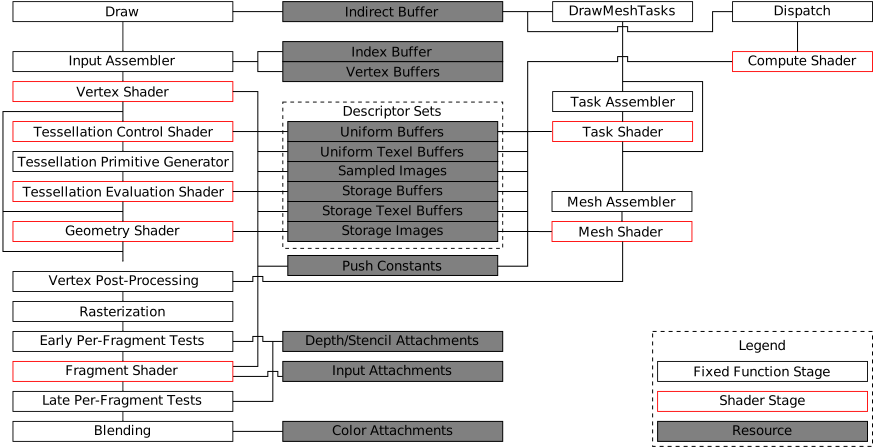
• Reference the full graphics pipeline when debugging a frame

  I had successfully submitted my draw call with a bound vertex buffer but the quad I had defined wasn’t being shaded. To debug this, I needed to know everything that happened after the vertex shader that would eventually lead to a fragment colour entering the framebuffer. The diagram and pages in references gave me that overview.

  Then it was a matter of looking at all the stages and operatons that could prevent my inputs from being shaded and written to the framebuffer. Things like clipping, discarding, blending. After checking all of these I eventually found that my issue was right at the end: my colour write mask was 0, so nothing was being written to the framebuffer.

• RenderDoc has performance counters built-in

  One of the first things I tested in debugging the above was whether any fragments were actually generated. If they weren’t, then the problem was something before my fragment shader. And if they were, then the problem was during or after my fragment shader. I used the performance counter viewer to capture PS Invocations (pixel shader invocations). I saw that there were many invocations, roughly one per pixel in my viewport. This demonstrated that no clipping or culling had occurred.

Next steps

• Render a cube in perspective

References

• The graphics pipeline:

  1. Pre-rasterization shader stages
  2. Fixed-function vertex post-processing
  3. Rasterization
  4. Fragment operations
  5. Framebuffer

  

Entry 5: More quads

2026-10-09

I’ve rendered two quads in perspective:

One quad is in front, and one behind. The camera is looking slightly down at them, which is why they’re stretched at the top.

My gl_DrawID trick from last entry worked; I had vkCmdDrawIndirect issue two draw calls against the same vertex buffer, and each draw call pulled a different transformation matrix from a storage buffer. I think it would be more correct to do this with instancing, though, seeing as it’s the same repeated.

What I built

• Use glm for matrix math
• Render a quad in perspective relative to a camera
• Use multi-draw indirect to render two quads
• Simplify feature selection for device creation

Next steps

• Load and render a mesh from a GLTF model

Entry 6: Loading a model

2026-10-10

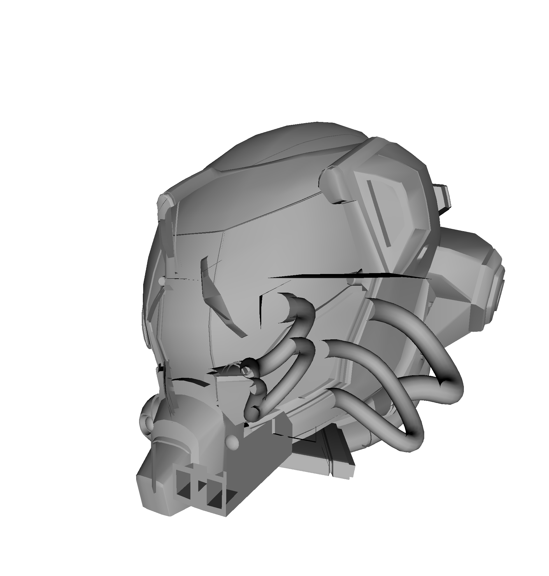
Finally, something decent on the screen! The only surprise was how well things worked on my first try. It was pretty straightforward to adapt my quad-rendering code to use the indices, positions, and normals provided by the GLB file.

What I built

• (Naively) load a model using tinygltf
• Render Damaged Helmet with diffuse reflection towards the camera
• Add scroll wheel zoom and hacky mouse drag rotation

What I learned

• vec3 is discouraged in shader uniforms

  https://stackoverflow.com/questions/38172696/should-i-ever-use-a-vec3-inside-of-a-uniform-buffer-or-shader-storage-buffer-o

  I found this while I was debugging layout issues in my camera uniform caused by adding the direction vector. It looks like the alignment for vec3 differs significantly between GLSL and C++.

Next steps

• Use a depth buffer
• Generalise model loading
• Fix rotation axis weirdness (my hacky mouse drag rotation is needs (0, 0, 1) to have the model rotate around the vertical axis (???))
• Implement non-hacky, natural mouse drag rotation

References

• https://www.khronos.org/files/gltf20-reference-guide.pdf
• https://registry.khronos.org/glTF/specs/2.0/glTF-2.0.html

Entry 7: Texturing

2026-10-11

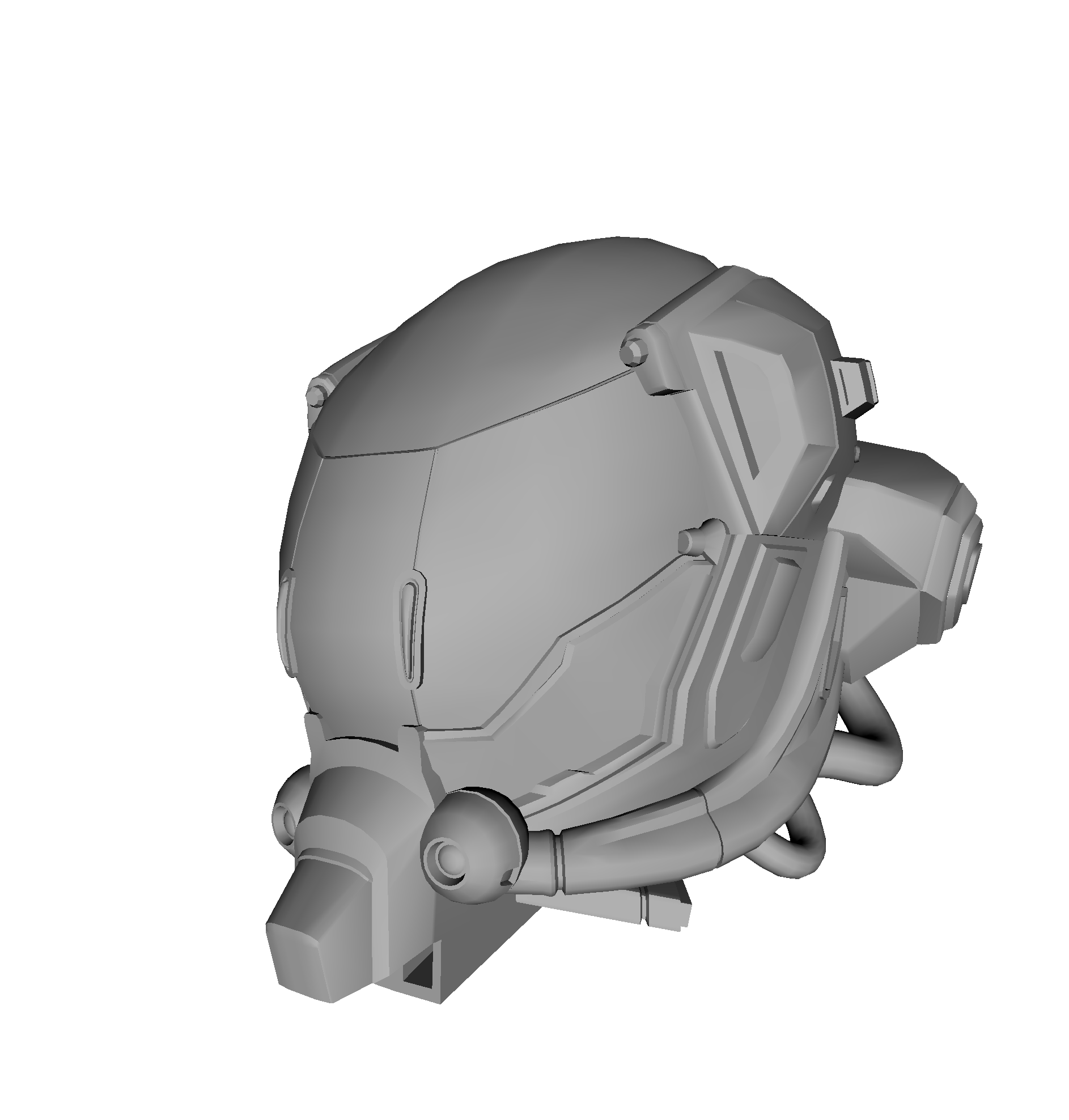
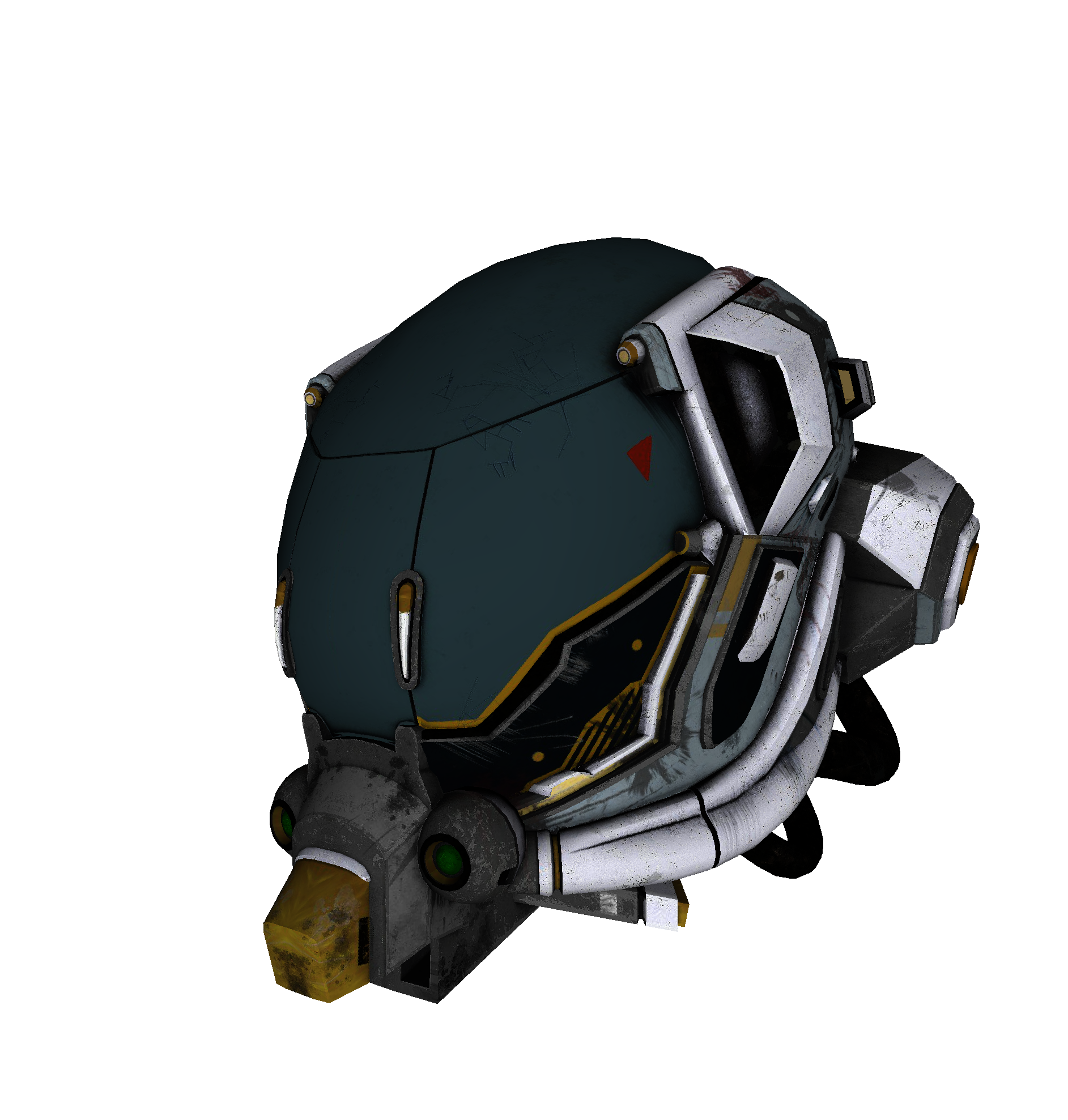
It’s starting to look cool :)

What I built

• Use depth buffer
• Fix and improve mouse drag rotation
• Sample base colour texture
• Started work on PBR materials

Next steps

• Generalise model loading (mostly put this off)
• Keep working on PBR materials

References

• https://docs.vulkan.org/guide/latest/depth.html
• https://docs.vulkan.org/spec/latest/chapters/samplers.html

Entry 8: PBR materials

2026-10-12

I made a first attempt at physically-based materials today. Here’s Damaged Helmet with a directional light from above:

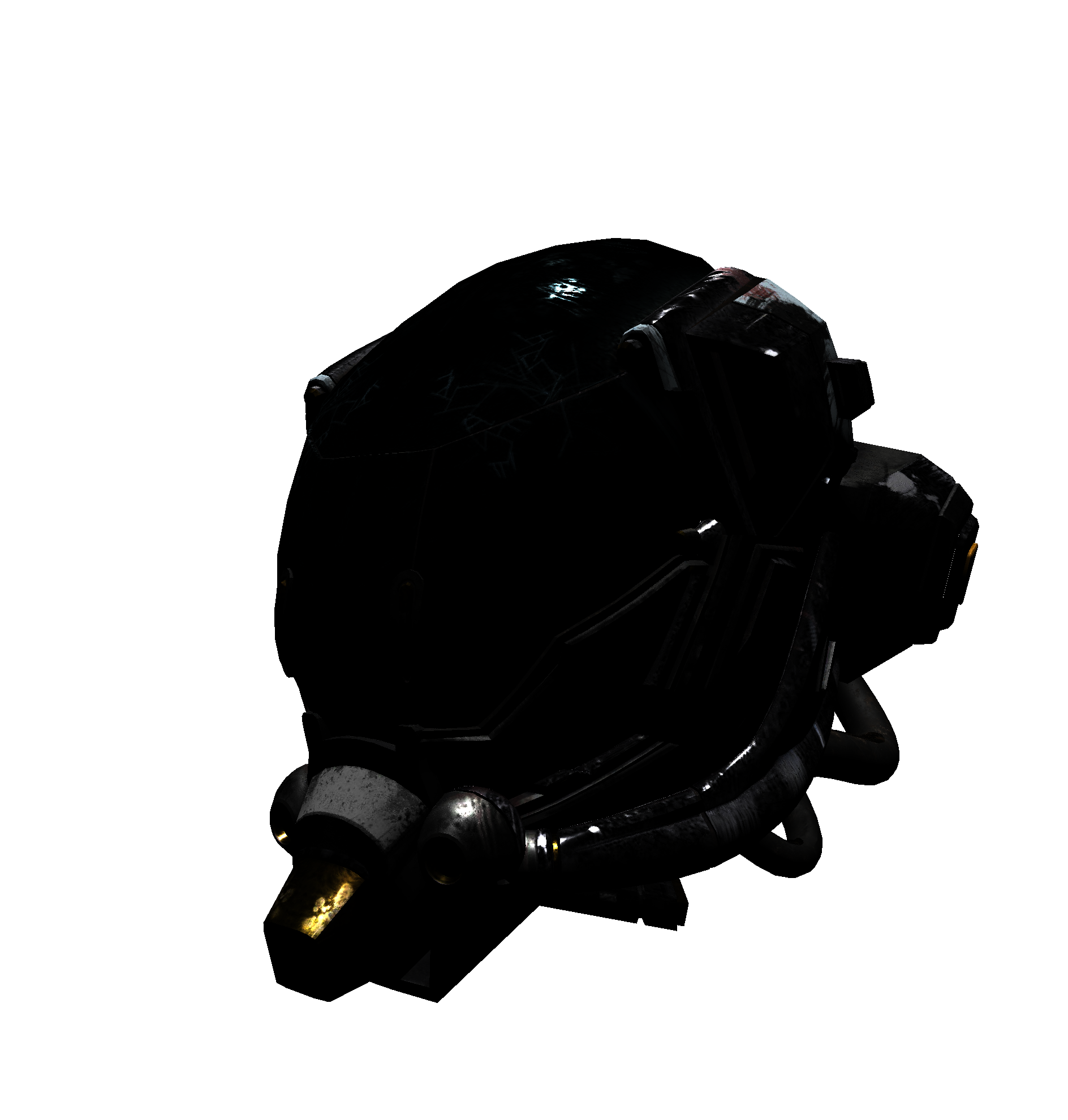
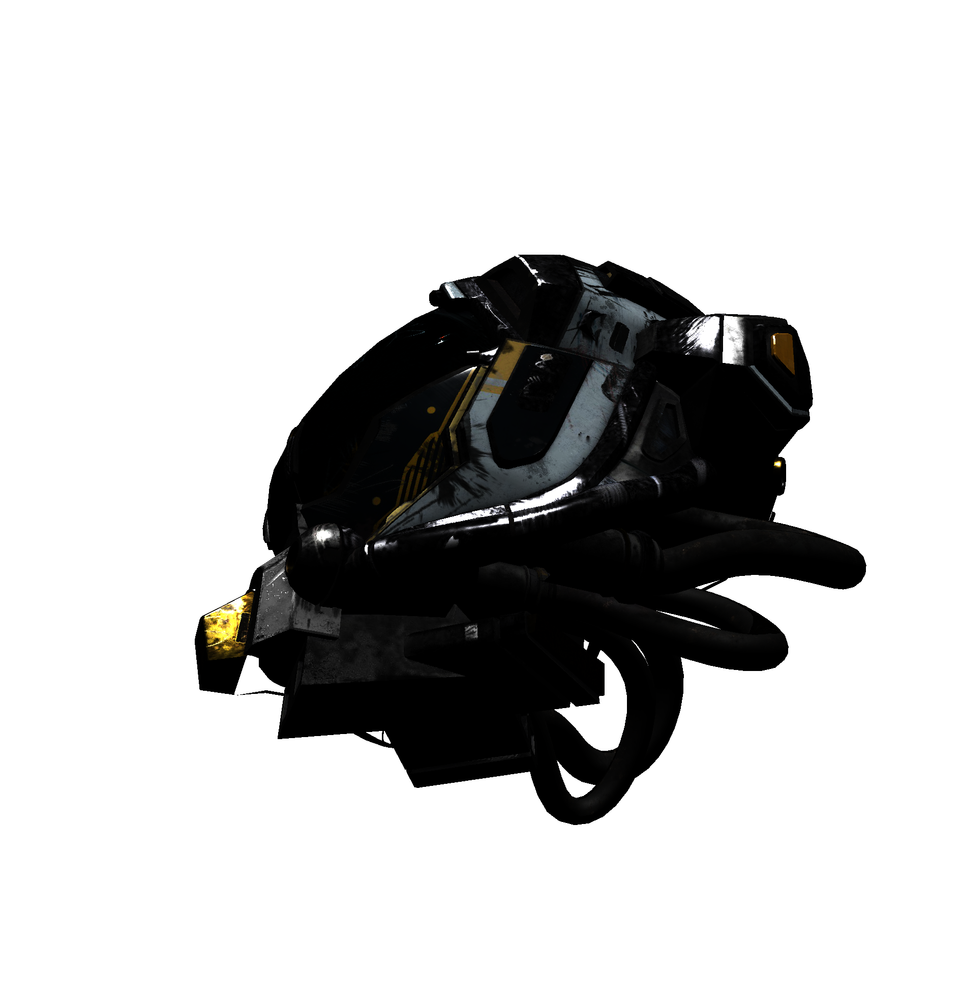
It doesn’t look very cool. I think the problem is that there’s no ambient light. The directional light illuminates the top of the model, so vertical surfaces reflect no light. If I rotate the model so that its side is facing up a bit, we can see that the shading is working:

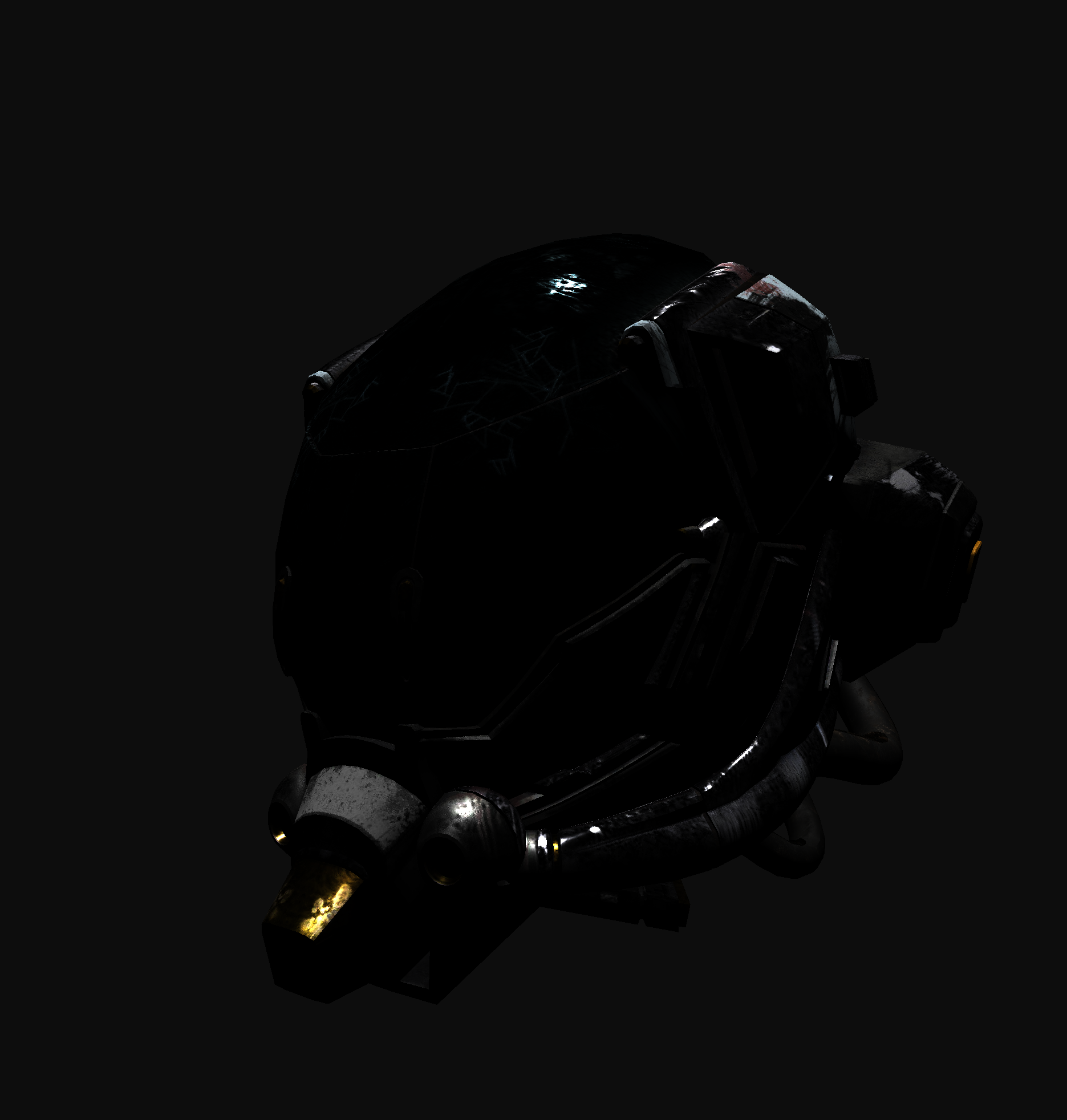
Another consequence of the lack of ambient light is that the metallic surfaces (such as the visor) barely read. I guess this is what the lighting situation would be if the model was in outer space with just the sun and no stars.

After I did this, I spent a lot of time learning about radiometry for computer graphics (see references) to understand how I should approach lighting beyond my simple directional light.

What I built

• Load the model’s metallic-roughness texture and sample it in the fragment shader
• Implement dielectric and metallic BDRFs
• Shade model with a directional light

Next steps

• Generalise model loading
• Shade with physical units
• Implement ambient lighting (either by full image-based lighting, or by adding ambient terms to the rendering equation)

References

• https://blog.selfshadow.com/publications/s2013-shading-course/hoffman/s2013_pbs_physics_math_notes.pdf
• https://cseweb.ucsd.edu/~viscomp/classes/cse168/sp26/readings/EGSR07-btdf.pdf
• https://pbr-book.org/4ed/Radiometry,_Spectra,_and_Color/Radiometry
• https://www.youtube.com/watch?v=5lGYm8L_rfo

Entry 9: Ambient diffuse

2026-10-13

Today I added ambient diffuse lighting.

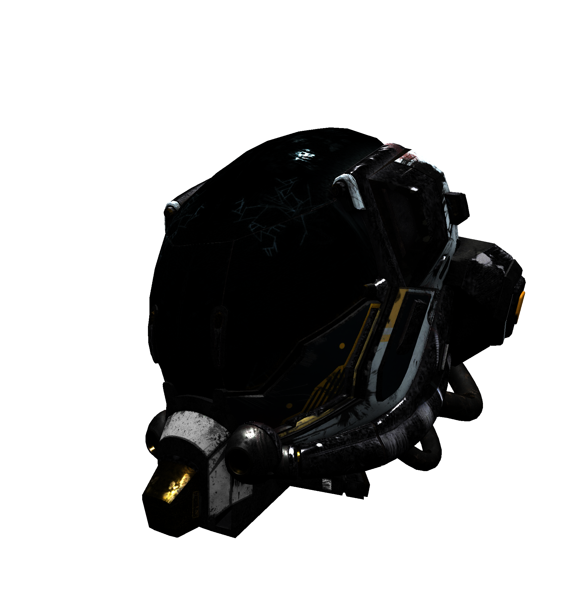
I basically did a whole lot of calculus to figure out that I just needed to add in a factor of the base colour for dielectric materials. After simplifying the rendering equation for the diffuse component of my dielectric BRDF, I was left with a multiplication by 1 - [an integral over the hemisphere, parameterised by dot(view vector, surface normal)]. I tried to approximate the integral with quadrature and when I plotted it for various values of dot(view vector, surface normal) I saw that it was small (0.01 - 0.03) over all angles, so I decided to leave it out.

Next, I want to add the ambient specular term. More integral simplification leads to the split-sum approximation (see references). In the case of ambient light it’s actually exact. There are two involved integrals to compute, parameterised over roughness and dot(view vector, surface normal). The split-sum approach precomputes the integral for various parameter values and stores them in a lookup table texture for use in the shader. I tried doing this with quadrature but the resulting texture seems off. I guess I should try using it just for fun. Apparently Monte Carlo integration with importance sampling is the right way to evaluate this integral. I find importance sampling less intuitive than quadrature, so I’ll spend a bit of time studing Monte Carlo integration to try and gain enough knowledge to implement the LUT generator myself.

Next steps

• Generalise model loading
• Shade with physical units
• Implement ambient specular term

References

• Real shading in Unreal Engine 4 (split-sum approximation)

Entry 10: Ambient specular

2026-10-14

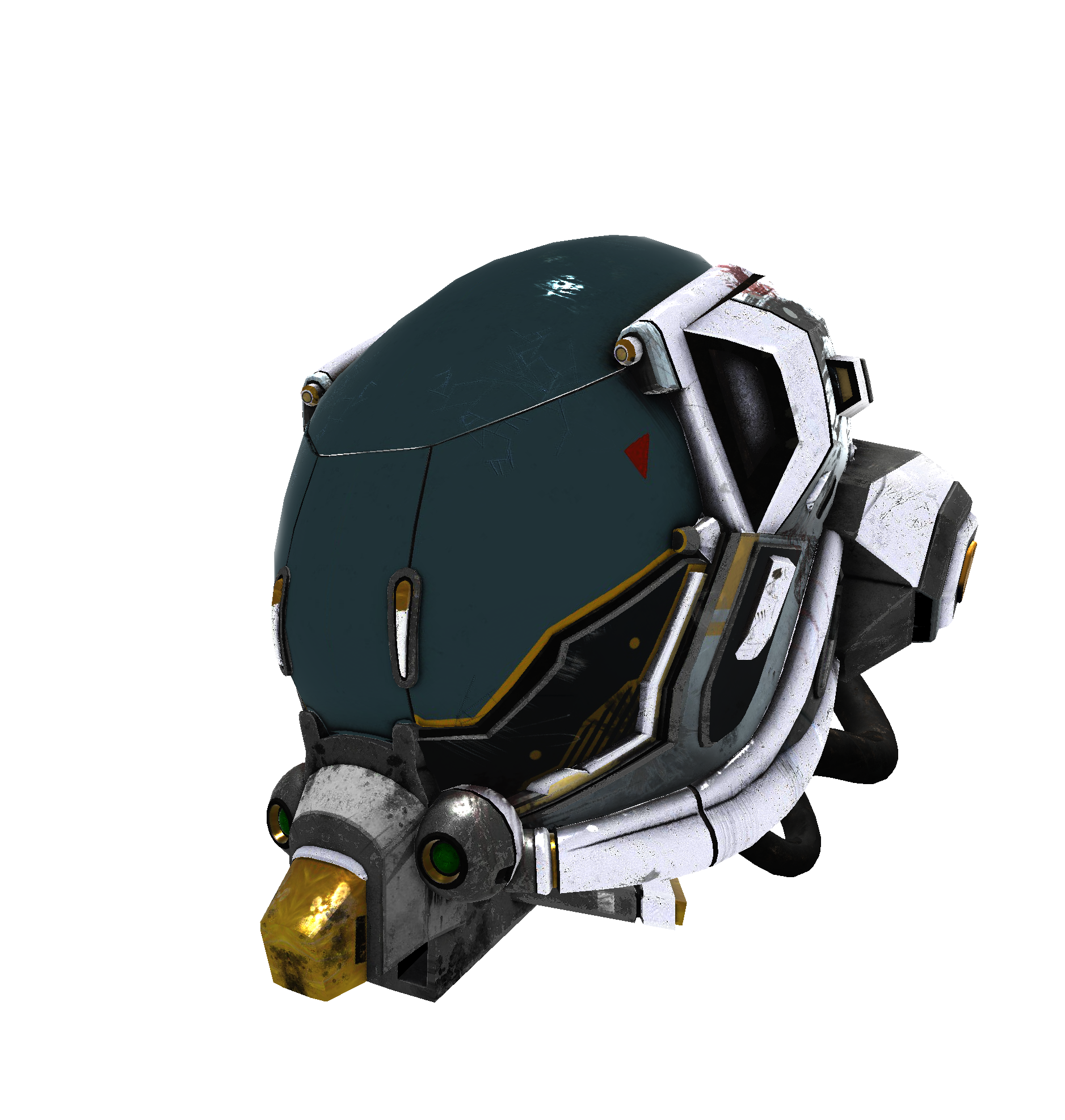
I’ve implemented an ambient specular term following the approach of Unreal Engine 4 (see references). I had to learn about numerical integration, Monte Carlo methods, importance sampling, and a little bit of vector calculus. My brain hurts! But it’s worth it:

Importance sampling a GGX BDRF for ambient specular radiance

$$f_r(\bar{i}, \bar{o}, \bar{n}) = \frac {F(\bar{i}, \bar{h}) G(\bar{i}, \bar{o}, \bar{h}) D(\bar{h})} {4(\bar{i} \cdot \bar{n})(\bar{o} \cdot \bar{n})}$$

where $\bar{h} = \frac{\bar{i} + \bar{o}}{|\bar{i} + \bar{o}|}$ is the halfway vector between $\bar{i}$ and $\bar{o}$. $f_r$ is implicitly parameterised over a roughness parameter.

The goal is solve the following integral

$$\int_\Omega L_i(\bar{i})f_r(\bar{i}, \bar{o}, \bar{n})(\bar{i} \cdot \bar{n}) d\omega_i$$

at a particular roughness and viewing angle $\bar{i} \cdot \bar{n}$.

I want to supply ambient light, which means constant direction-independent radiance:

$$L_i(\bar{i}) = \text{Ambient}$$

The integral simplifies to

$$\text{Ambient} \int_\Omega f_r(\bar{i}, \bar{o}, \bar{n})(\bar{i} \cdot \bar{n}) d\omega_i$$

Inline $f_r$ and the $\bar{i} \cdot \bar{n}$ terms cancel

$$\text{Ambient} \int_\Omega \frac {F(\bar{i}, \bar{h}) G(\bar{i}, \bar{o}, \bar{h}) D(\bar{h})} {4(\bar{o} \cdot \bar{n})} d\omega_i$$

I’m using Schlick’s approximation for $F$

$$\begin{aligned} F(\bar{i}, \bar{h}) & = F_0 + (1 - F_0)(1 - (\bar{i} \cdot \bar{h}))^5 \\ & = F_0 + (1 - (\bar{i} \cdot \bar{h}))^5 - F_0(1 - (\bar{i} \cdot \bar{h}))^5) \\ & = F_0 - F_0(1 - (\bar{i} \cdot \bar{h}))^5) + (1 - (\bar{i} \cdot \bar{h}))^5 \\ & = F_0(1 - (1 - (\bar{i} \cdot \bar{h}))^5) + (1 - (\bar{i} \cdot \bar{h}))^5 \end{aligned}$$

Which splits the integral into two parts

$$\text{Ambient} \lparen F_0 \int_\Omega \frac {(1 - (1 - (\bar{i} \cdot \bar{h}))^5) G(\bar{i}, \bar{o}, \bar{h}) D(\bar{h})} {4(\bar{o} \cdot \bar{n})} d\omega_i + \int_\Omega \frac {(1 - (\bar{i} \cdot \bar{h}))^5 G(\bar{i}, \bar{o}, \bar{h}) D(\bar{h})} {4(\bar{o} \cdot \bar{n})} d\omega_i \rparen$$

When I try to estimate these integrals with Monte Carlo integration I get poor results for small roughness values. The estimates have very high variance. My intuitive guess for this is that at low roughness, the microfacet normals converge on the surface normal, so the radiance will only be propagated from directions near the reflection of $\bar{v}$ around $\bar{n}$, of which there are very few.

The typical solution is to sample from the hemisphere around $\bar{h}$ using a distribution based on $D$.

These two integrals have the general shape

$$\int_\Omega \frac {\text{stuff}(\bar{i}, \bar{o}, \bar{h})} {4(\bar{o} \cdot \bar{n})} D(\bar{h}) d\omega_i$$

Monte Carlo integration says that

$$\frac{1}{N} \sum_i^N f(\bar{x}_i) \approx \int_\Omega f(\bar{x}) p(\bar{x}) d\omega_x$$

when $\bar{x}_i$ are sampled according to the PDF $p$.

Our integral can be rearranged into this form. $D(\bar{h})(\bar{n} \cdot \bar{h})$ is a PDF, so

$$\int_\Omega \frac {\text{stuff}(\bar{i}, \bar{o}, \bar{h})} {4(\bar{o} \cdot \bar{n})(\bar{n} \cdot \bar{h})} D(\bar{h})(\bar{n} \cdot \bar{h}) d\omega_i$$

Now we have to change the integral from solid angles around $\bar{i}$ to solid angles around $\bar{h}$.

We have $\bar{i} = 2(\bar{o} \cdot \bar{h})\bar{h} - \bar{o}$ (derived from the definition of $\bar{h}$) and $d\omega_i = 4(\bar{o} \cdot \bar{h}) d\omega_h$ (which is required for the change of variables, but I don’t understand how to derive it yet) (EDIT: the “Roughness Using Microfacet Theory” section in PBRT has a good explanation of this quantity]).

This gives

$$\begin{aligned} & \int_\Omega \frac {\text{stuff}(\bar{i}, \bar{o}, \bar{h})} {4(\bar{o} \cdot \bar{n})(\bar{n} \cdot \bar{h})} D(\bar{h})(\bar{n} \cdot \bar{h}) 4(\bar{o} \cdot \bar{h})d\omega_h \\ = & \int_\Omega \frac { (\bar{o} \cdot \bar{h}) \text{stuff}(\bar{i}, \bar{o}, \bar{h}) } {(\bar{o} \cdot \bar{n})(\bar{n} \cdot \bar{h})} D(\bar{h})(\bar{n} \cdot \bar{h}) d\omega_h \end{aligned}$$

where $\bar{i}$ is now defined in terms of $\bar{o}$ and $\bar{h}$.

Walter et al. (2007) give equations for sampling $\bar{h}$ from a particular $D(\bar{h})(\bar{h} \cdot \bar{n})$. If we use those, then

$$\frac{1}{N} \sum_k^N \frac { (\bar{o} \cdot \bar{h_k}) \text{stuff}(\bar{i}, \bar{o}, \bar{h_k}) } {(\bar{o} \cdot \bar{n})(\bar{n} \cdot \bar{h_k})} \approx \int_\Omega \frac { (\bar{o} \cdot \bar{h}) \text{stuff}(\bar{i}, \bar{o}, \bar{h}) } {(\bar{o} \cdot \bar{n})(\bar{n} \cdot \bar{h})} D(\bar{h})(\bar{n} \cdot \bar{h}) d\omega_h$$

Next steps

• Clean up my LUT generator and add to the project
• Generalise model loading
• Shade with physical units

References

• Generating uniformly distributed numbers on a sphere – Mathemathinking
• Importance Sampling - YouTube
• Rendering Lecture 06 - Importance Sampling - YouTube
• What is Jacobian? | The right way of thinking derivatives and integrals - YouTube
• Microfacet Models for Refraction through Rough Surfaces (2007)
• Real Shading in Unreal Engine 4 (2013)

Entry 11: Playing around

2026-10-15

I spent most of my time learning more about vector calculus and Jacobian matrics and their determinants in an attempt to understand the $d\omega_i = 4(\bar{o} \cdot \bar{h}) d\omega_h$ that came up yesterday. I tried to apply what I learned but I couldn’t get close to the answer. Then I found a good explanation in the “Roughness Using Microfacet Theory” section in PBRT. Here’s how I understand it now:

Consider the unit hemisphere with $\bar{o}$ as the pole. $\bar{i}$ and $\bar{h}$ are also directions in this hemisphere, with spherical coordinates $(\theta_i, \phi_i)$ and $(\theta_h, \phi_h)$ respectively. $\bar{h}$ is halfway between $\bar{o}$ and $\bar{i}$, but because $\bar{o}$ is the pole, $\bar{h}$ and $\bar{i}$ share the same azimuthal angle. So we have $\theta_i = 2\theta_h$ and $\phi_i = \phi_h$.

The Jacobian we’re looking for is

$$\frac{d\omega_h}{d\omega_i} = \frac {\text{sin}(\theta_h)d\theta_{h}d\phi_h} {\text{sin}(\theta_i)d\theta_{i}d\phi_i}$$

$\phi_i = \phi_h$ implies $d\phi_i = d\phi_h$, and $\theta_i = 2\theta_h$ implies $d\phi_i = 2d\phi_h$, giving

$$\begin{aligned} \frac{d\omega_h}{d\omega_i} & = \frac {\text{sin}(\theta_h)d\theta_{h}d\phi_h} {\text{sin}(2\theta_h)2d\theta_{h}d\phi_h} \\ & = \frac {\text{sin}(\theta_h)} {2\text{sin}(2\theta_h)} \\ & = \frac {\text{sin}(\theta_h)} {4\text{sin}(\theta_h)\text{cos}(\theta_h)} \\ & = \frac{1}{4\text{cos}(\theta_h)} \\ & = \frac{1}{4(\bar{o} \cdot \bar{h})} \end{aligned}$$

At the end of the day I tried loading a different model, and the program crashed because I forgot that my code is specialised to the Damaged Helmet model. So general GLTF loading definitely next on the list.

What I built

• Simplified descriptor set management
• Pass a GLB file on the command line

Next steps

• Clean up my LUT generator and add to the project
• Generalise model loading
• Shade with physical units

Entry 12: Generic model loading

2026-10-16

I’m generalising my GLTF loader to work with arbitrary models. One problem I’ve run into is binding the material textures at the right time. A mesh has many primitives, and each primitive has a material. The material can reference textures for properties like base colour and metallic-roughness, which are used in the fragment shader. Until now I had set all this up at the start of the program, because I was using a model with a single mesh that contained a single primitive. But now that I want to work with an arbitrary number of primitives, I need to allow the material properties to change during a render pass.

I think the traditional way to handle this is to have a separate descriptor set layout for material properties, and create a descriptor set with that layout per material. To render, loop over all primitives and bind the material descriptor set before drawing the primitive. But I don’t like it, because it’s not compatible with draw-indirect.

A draw-indirect friendly version needs use gl_DrawID to lookup the material texture for the fragment. For data like per-object transforms, I just index into a storage buffer, but I can’t do that for samplers or textures. There are descriptor arrays, but they seem like a hack. A dynamic texture atlas looks like the right way to do it, but it’s a lot of work.

For now, I’ve just gone with the traditional way to get the model loader working. Later on I can figure out how to make it draw-indirect-compatible.

Next steps

• Keep working on generalised model loading
• Shade with physical units

Entry 13: Loading a second model

2026-10-17

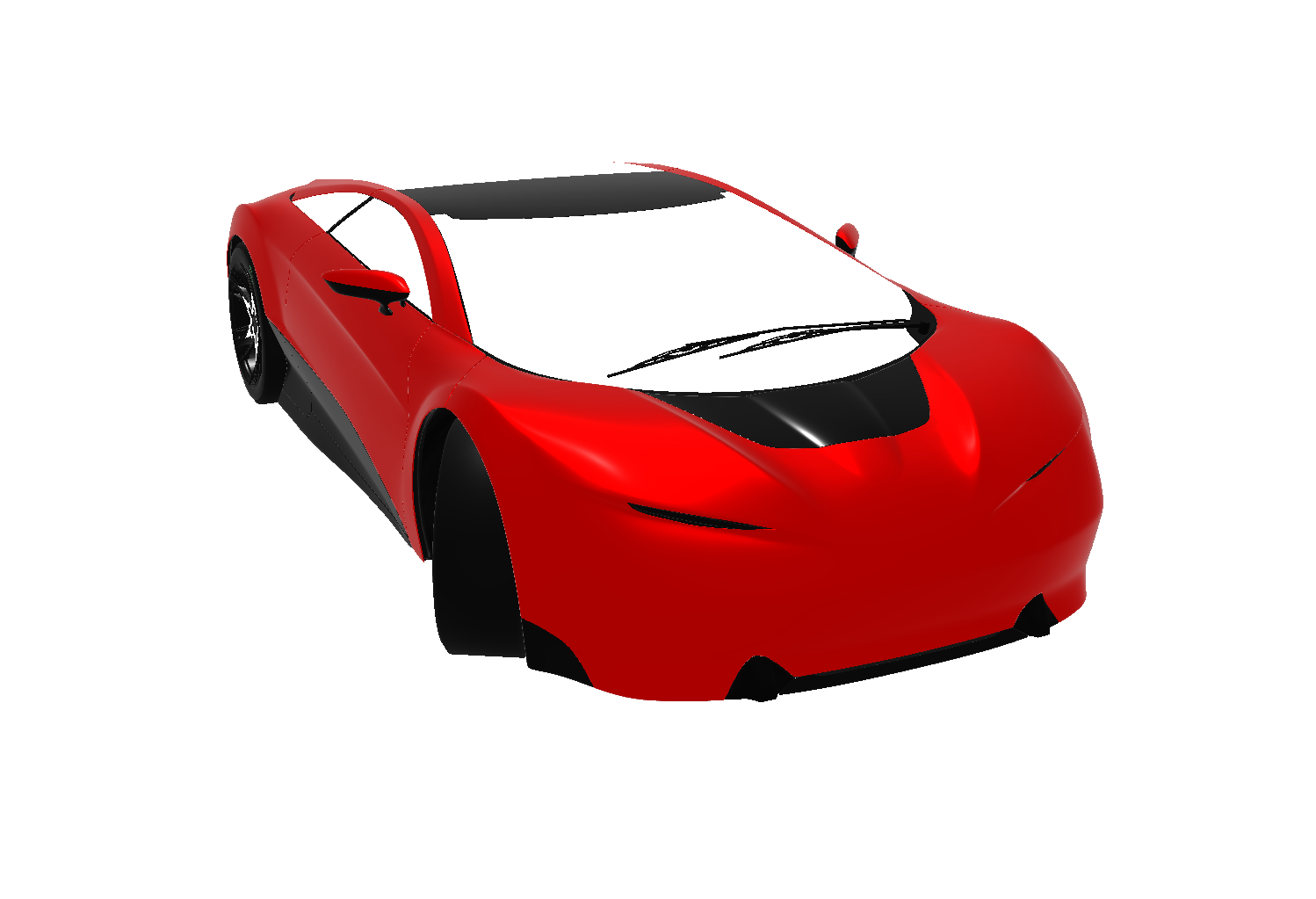
I’ve generalised model loading enough to load a second model: Car Concept. The most obvious thing mine lacks is support for transparent materials.

What I learned

• Negative dot products can appear during rendering

  I noted that certain areas became black when facing certain directions. It was when they faced away from the directional light, so the dot product of the normal with the direction-toward-the-light was negative. This removed colour from the fragment.

• Normals need to be transformed differenly to positions

  When I first got the car loaded, reflections on different parts looked wrong. For example, some parts had extreme fresnel reflection when facing the camera instead of at grazing angles. I realised that the normals passed to the fragment shader were wrong, but I didn’t know why. I changed the fragment shader to colour the model using its normals, and compared the transformed and untransformed normals. Untransformed normals looked smooth, but the transformed normals were inconsistent across parts of the car. This suggested that my transform was causing issues.

  I did some searching about transforming normals, and I found out that using the position transform on normals is incorrect in general. The usual way to transform normals is to take the transposed inverse of the position transformation matrix. While reading about this, I learned that the cofactor matrix is a more correct way to transform normals, so I implemented that.

Next steps

• Test with more models
• Review/clean up model loading code
• Shade with physical units

References

• https://terathon.com/blog/transforming-normals.html
• https://github.com/graphitemaster/normals_revisited

← Local Hoogle Newest