Still working things out. There’s a lot of theory behind the switch to proper physical units. Hopefully I can write some code soon!

A physically-based camera

To measure power from the scene, we need a physically-based camera. Light passes through an aperture (usually circular), then a system of lenses that focus the light down to a point. When the subject is infinitely far away, the light rays coming from it are parallel, and are converged by the lens at a distance known as the focal length. It’s at this plane that the image is formed on the sensor.

I had a lot of trouble trying to go from this definition of a camera to the energy measured by the sensor. The Wikipedia article on F-number gives the following equation for the irradiance $E$ (actually, illuminance) in terms of incident radiance $L$ (actually, luminance):

$$E = L\frac{\pi}{4N^2}$$

where $N = \frac{f}{D}$, $f$ is the focal length, and $D$ is the aperture’s diameter.

According to the units, $\frac{\pi}{4N^2}$ must be a solid angle. But how was it derived?

Substituting $N$, we get

$$E = L\frac{\pi{D}^2}{4f^2}$$

I spy the area of the aperture: $\pi(\frac{D}{2})^2$. The formula for solid angle is $\Omega = \frac{A}{r^2}$, where $A$ is the area of a region on a sphere, and $r$ is the radius of the sphere. So $\frac{\pi{D}^2}{4f^2} = \frac{\pi(\frac{D}{2})^2}{f^2}$ is the solid angle subtended by a region with area equal to that of the aperture on a sphere with radius equal to the focal length.

But the aperture is a flat disc, not a curved spherical cap. So how is this a valid solid angle? I think it’s fine, assuming that the aperture is very small compared to the focal length:

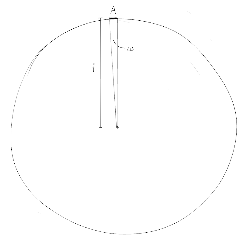
However, this is only accurate for radiance coming straight at the aperture. The error increases for radiance at oblique angles. To account for this, we first need to use the aperture’s projected area $A'$ instead of its actual area $A$: $A' = A\cos\theta$ ($\theta$ is the angle between the aperture’s normal and the radiance’s direction). Then we need the correct sphere radius. A line of length $r$ from the aperture to the focus plane only has $r = f$ when it’s perpendicular to the focus plane. Otherwise, this line hits the plane at an angle, becoming the hypotenuse of a right triangle, one side of which is $f$. The angle between $r$ and $f$ is $\theta$, so $r = \frac{f}{\cos\theta}$. Putting it all together:

$$\Omega = \frac{A'}{r^2} = \frac{A\cos\theta}{(\frac{f}{\cos\theta})^2} = \frac{A\cos^3\theta}{f^2}$$

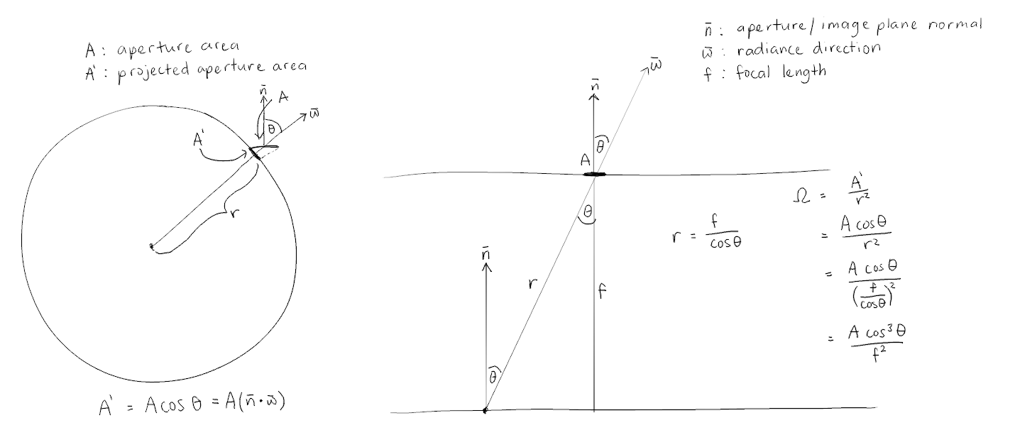
Now we have

$$E = L\frac{\pi{D}^2\cos^3\theta}{4f^2} = L\frac{\pi{\cos}^3\theta}{4N^2}$$

for irradiance at a point on the focal plane.

There’s one last step, though. The above equation gives the irradiance at that point for a surface perpendicular to the direction of the incoming radiance. To get the irradiance for the surface at that point, we need to project the area of the radiance’s implicit surface onto the focal plane. This adds another $\cos\theta$ factor:

$$E = L\frac{\pi{D}^2\cos^4\theta}{4f^2} = L\frac{\pi{\cos}^4\theta}{4N^2}$$

This gives the $\cos^4\theta$ factor defined in this more advanced version of the camera equation. This factor contributes to vignetting.

We’ve handled the solid angle, but what about the area? $E$ is irradiance ($Wm^{-2}$), so do I have to multiply it by some area to get power? Apparently not. Every pixel in the framebuffer is analogous to a pixel in a camera sensor. Integrating the irradiance over time gives radiant exposure ($Jm^{-2}$). The energy collected by the pixel is the average radiant exposure over the pixel multiplied by its area, so the measured energy is proportional to the radiant exposure. For the purposes of rendering, we care about the relationships between the measurements at each pixel (e.g. this pixel is darker/lighter than that other one) rather than the values themselves. In other words, once we have radiant exposure, we will render the scene the same way regardless of the choice of pixel size.

The f-number $N$ together with the exposure time $t$ determine the radiant exposure of an image. How do we choose values for these two parameters? It depends on the sensor’s film speed.

At the start of an exposure, the sensor reports black everywhere. Then, as photons are received, sensor levels grow until they reach some maximum threshold which corresponds to white. For digital sensors the level is a charge, and for film it’s the number of exposed grains in a small area. Film speed sets the threshold that corresponds to maximum exposure/white. I’ll use ISO saturation-based speed because it seems easiest to implement:

$$S_{sat} = \frac{78}{H_{sat}}$$

where $S_{sat}$ is the saturation-based ISO, and $H_{sat}$ is the maximum radiant exposure (the white level).

We can express $H_{sat}$ in terms of $S_{sat}$, $N$ and $t$:

$$\begin{aligned} H_{sat} & = \frac{78}{S_{sat}} \\ L_{sat}\frac{\pi}{4N^2}t & = \frac{78}{S_{sat}} \\ \frac{\pi}{4N^2}t & = \frac{78}{S_{sat}L_{sat}} \end{aligned}$$

I’ve used $\cos\theta = 1$ here because that’s where we’ll get maximum radiant exposure. $L_{sat}$ is the radiance that will register as white given a choice of $S_{sat}$, $N$ and $t$.

$S_{sat}$ and $L_{sat}$ are fixed for a scene, leaving two unknowns. The solution to this equation is a line; there are an infinite number of $(N, t)$ combinations that let the same amount of light in. For this reason, photographers use exposure value (EV) to represent the equivalence class of $(N, t)$:

$$EV = \log_2(\frac{N^2}{t}) = 2\log_2(N) - \log_2(t)$$

I found it odd that a larger EV means less exposure, but it just means that you use higher EV settings for a brighter scene.

Since the effects of f-number and exposure time (depth of field and motion blur, respectively) generally aren’t captured by the camera in a real-time renderer, let’s rewrite the exposed camera equation in terms of EV:

$$\begin{aligned} EV & = \log_2(\frac{N^2}{t}) \\ 2^{EV} & = \frac{N^2}{t} \\ 2^{-EV} & = \frac{t}{N^2} \end{aligned}$$

Giving

$$H = L\frac{\pi{\cos}^4\theta}{4}2^{-EV}$$

We can also rewrite the film speed equation in terms of EV. That reduces the equation from two variables to one, giving the EV to use for film speed $S$ such that a certain radiance $L_{sat}$ will expose to white:

$$\begin{aligned} \frac{\pi}{4N^2}t & = \frac{78}{SL_{sat}} \\ \frac{t}{N^2} & = \frac{4}{\pi}\frac{78}{SL_{sat}} \\ \frac{N^2}{t} & = \frac{\pi}{4}\frac{SL_{sat}}{78} \\ \log_2(\frac{N^2}{t}) & = \log_2(\frac{\pi}{4}\frac{SL_{sat}}{78}) \\ EV_{S} & = \log_2(\frac{\pi}{4}\frac{SL_{sat}}{78}) \end{aligned}$$

When an equation like the above is used to calculate an EV, and then use that EV in the modified camera equation to produce radiant exposure, we’re performing automatic exposure. The renderer will record radiance at each pixel in the framebuffer, use those radiances to produce an appropriate $L_{sat}$, calculate $EV_S$, then map radiance to radiant exposure based on that $EV_S$. Now, what’s an appropriate $L_{sat}$ for a frame?

You could use the maximum radiance, but that would allow a single outlier pixel to determine the exposure of the entire image. Imagine a frame that’s mostly dark due to being exposed for small, extremely bright specular highlight. Using a percentile (say, 95th percentile) for $L_{sat}$ would be better than the maximum. It seems a bit weird to essentially expose for a certain amount of clipping, though.

The references I’ve seen so far calculate an EV that exposes the average radiance (or a weighted average) to a “medium tone” (e.g. middle grey). https://en.wikipedia.org/wiki/Light_meter#Exposure_equations gives:

$$\frac{N^2}{t} = \frac{L_{avg}S}{K}$$

where $K$ is a “light meter calibration constant”. To compute the corresponding EV:

$$\begin{aligned} \frac{N^2}{t} & = \frac{L_{avg}S}{K} \\ \log_2(\frac{N^2}{t}) & = \log_2(\frac{L_{avg}S}{K}) \\ EV_S & = \log_2(\frac{L_{avg}S}{K}) \end{aligned}$$

If we take the common value $K = 12.5$, what do we learn about the relationship between $L_{sat}$ and $L_{avg}$?

$$\begin{aligned} EV_S = \log_2(\frac{L_{avg}S}{12.5}) & = \log_2(\frac{\pi}{4}\frac{SL_{sat}}{78}) \\ \frac{L_{avg}S}{12.5} & = \frac{\pi}{4}\frac{SL_{sat}}{78} \\ \frac{L_{avg}}{12.5} & = \frac{\pi}{4}\frac{L_{sat}}{78} \\ \frac{L_{avg}}{L_{sat}} & = \frac{\pi}{4}\frac{12.5}{78} \approx 0.126 \end{aligned}$$

That’s consistent with Wikipedia’s description of saturation-based speed:

The factor 78 is chosen such that exposure settings based on a standard light meter and an 18-percent reflective surface will result in an image with a grey level of $\frac{18\%}{\sqrt{2}} = 12.7\%$ of saturation.

So here’s my current plan:

1. For each fragment, store $L$ in the colour attachment l
2. Compute $L_{avg}$ from l
3. Compute $2^{EV_100} = \frac{100}{12.5}L_{avg} = 8L_{avg}$
4. For each $L$ in l, compute the normalised sensor level $\frac{H}{H_{sat}} = \frac{100}{78}L\frac{\pi\cos^4\theta}{4}\frac{1}{8L_{avg}} = L\frac{100\pi\cos^4\theta}{78 \cdot 4 \cdot 8 \cdot L_{avg}} = 0.126\frac{L}{L_{avg}}cos^4\theta$

If I use $L_{avg}$ from the previous frame, which seems reasonable to try at 60FPS, then I can collapse this into a single render pass.

There’s still another step required before the result can be written to a colour attachment. The normalised sensor levels are still in the range $[0, \infty)$, they’re just scaled so that $\ge 1$ means “saturated”. There are many ways to clamp this to $[0, 1]$ before writing to an sRGB buffer. But before I get to that (in another post), some notes about photometric units.

Photometry

In this post and the previous one I’ve been using radiometric units, but they aren’t the best units for a renderer. Radiant flux accounts for all electromagnetic radiation, but we can only see a small fraction of the spectrum. Regular camera sensors are also built to be sensitive to the visible spectrum. Therefore a renderer doesn’t need to model invisible radiation either. The subset of radiometry concerned with visible light only is called photometry.

A lumen ($lm$) is the photometric equivalent of a watt. Instead of measuring total power, it measures power of visible light. The eye is not equally sensitive to all wavelengths, so there are functions from wavelength to “luminous efficiency” ($lm/W$) that record how much of the incoming energy the eye picks up on. For example, 555nm light has approximately twice the lumious efficiency of 510nm light, and about ten times the luminous efficiency of 465nm light. So for a 555nm light source and a 465nm light source to appear similarly bright, the latter must output 10x as much power as the former.

All the other radiometric units have photometric equivalents, too. Here’s a table of the ones I’m interested in so far:

From now on I’ll use photometric units when appropriate.

References

• https://photographylife.com/exposure-value
• https://seblagarde.wordpress.com/wp-content/uploads/2015/07/course_notes_moving_frostbite_to_pbr_v32.pdf
• https://google.github.io/filament/Filament.md.html#imagingpipeline/physicallybasedcamera/automaticexposure
• https://en.wikipedia.org/wiki/Light_meter
• https://en.wikipedia.org/wiki/Photometry_(optics)
• https://www.johndcook.com/wavelength_to_RGB.html
• Sharpe, L. T., Stockman, A., Jagla, W., & Jägle, H. (2005). A luminous efficiency function, V*(λ), for daylight adaptation. Journal of vision, 5(11), 3-3.

← Sunstone dev log 21: radiometry musings Newest